Reading KL Divergence as a Subtraction: Displacement, Asymmetry, and the Log-Likelihood View
Brando Miranda — October 2026 · ~14 min read (+28 min appendix)
TL;DR. KL divergence gets taught with several personalities (extra bits, cross-entropy minus entropy, “relative entropy,” a “divergence” that is not a distance), and for years each one felt like its own thing to me. This post builds one grammar for all of them. Start with what we trust: \(B - A\) is the displacement of \(B\) from \(A\). Read \(D_{\mathrm{KL}}(p \Vert q)\) the same way, as \(p \mathbin{-^{\mathrm{KL}}_{p}} q\): the divergence of \(p\) from \(q\), with baseline \(q\), measured on samples from \(p\). Unroll it and it really is a subtraction: \(\mathbb{E}_{X \sim p}[\log p(X) - \log q(X)]\), the average log-likelihood gap between the two models on \(p\)’s own data. Pointwise, that gap flips sign when you swap \(p\) and \(q\), exactly like \(B - A = -(A - B)\). All of KL’s asymmetry comes from which distribution you average under, which is why I put it in the notation. The view is not new as math (Kullback and Leibler motivated KL exactly this way in 1951), but in 14 years of ML I had never seen it taught first, and I think it should be. This is the first post in a series on thinking about ML with less arbitrariness.
Why KL felt arbitrary to me
I’ve been doing machine learning since 2012. I have used KL divergence in losses, in bounds, in RL regularizers, in variational inference. And every time I met it, it showed up wearing a different outfit:
- the excess bits you pay for coding data from \(p\) with a code built for \(q\);
- cross-entropy minus entropy, \(H_p(q) - H_p(p)\), with minus signs everywhere;
- a “divergence,” which we are told is like a distance, except when it isn’t.
Each version is correct. What bothered me is that I had to switch mental models depending on the textbook, and the signs never felt natural. I want something less arbitrary: one notation, one picture, and every classical formula falls out of it. That’s the goal of this series, and KL is the first test case.
In my score matching post I subscripted the Fisher divergence with the distribution carrying the expectation and said I’d write the KL divergence the same way if I could rewrite the textbooks. This post does that, and it turns out the subscript is the whole story of the asymmetry.
Start with what we trust: \(B - A\)
Two points \(A\) and \(B\). The vector
\[B - A\]is the displacement of \(B\) from \(A\): start at \(A\), travel to \(B\). The thing you subtract is your baseline, where you start. Its length is the ordinary distance,
\[d(A, B) \;=\; \Vert B - A \Vert_2 .\]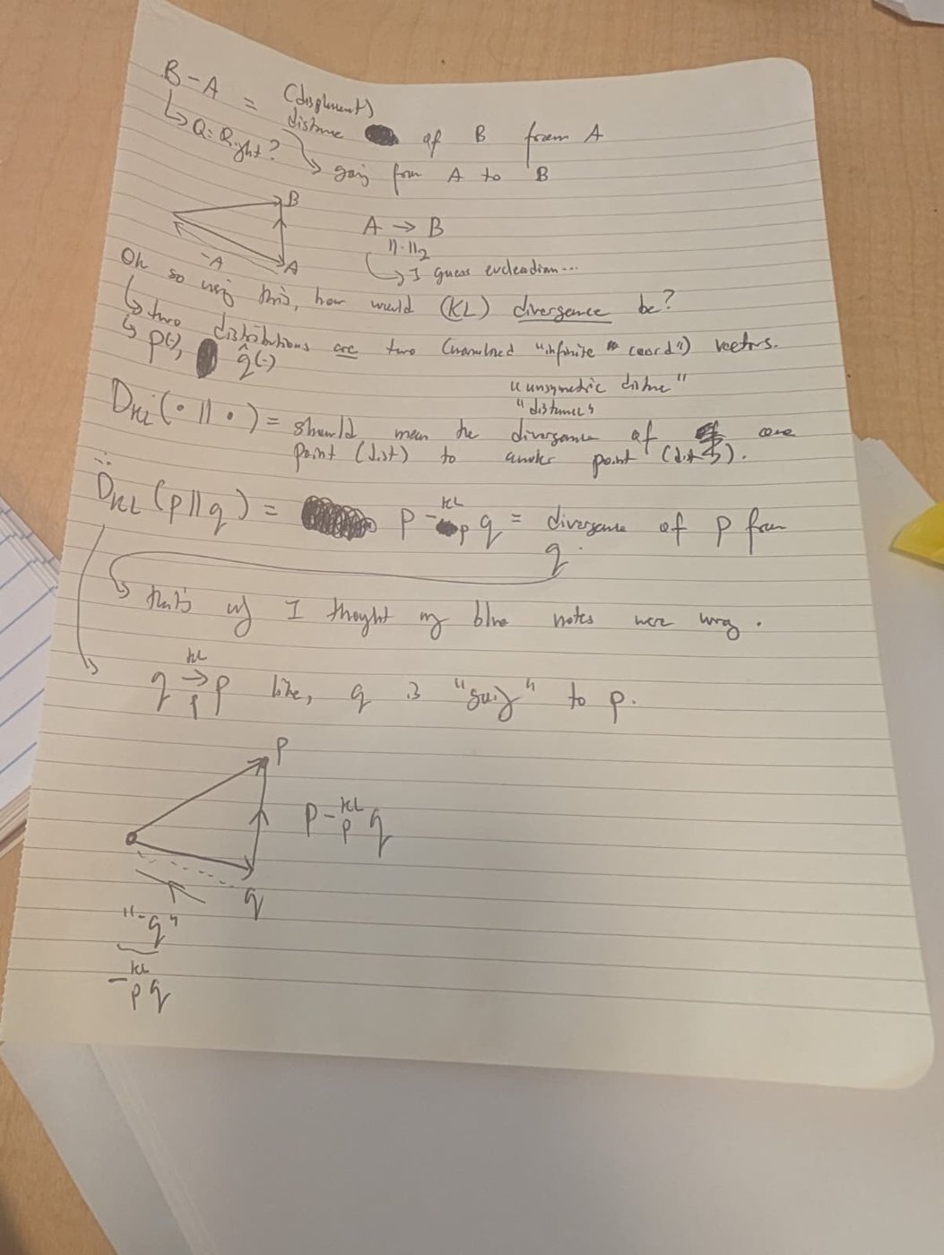
Everything we like about distances is visible here. The length is nonnegative and zero only when \(A = B\). It is symmetric, because \(A - B = -(B - A)\) and the norm forgets the sign. And it obeys the triangle inequality. Hold on to the sign-flip fact: the displacement is antisymmetric, the length is symmetric. That split is going to explain KL.
Distributions as points
Now take two distributions \(p\) and \(q\) over the same space \(\mathcal{X}\). Think of each as a point. On a discrete space, \(p \in [0,1]^{\mathcal{X}}\) is a vector with one coordinate per outcome \(x\), the coordinate being \(p(x)\), normalized so the coordinates sum to one. In the continuous case it’s an “infinite vector” indexed by \(x\): a density with \(\int p(x)\, dx = 1\). This is an analogy, not a theorem, but it suggests the question: what is the displacement of \(p\) from \(q\)?
Here is the notation I’ll use for the rest of the series:
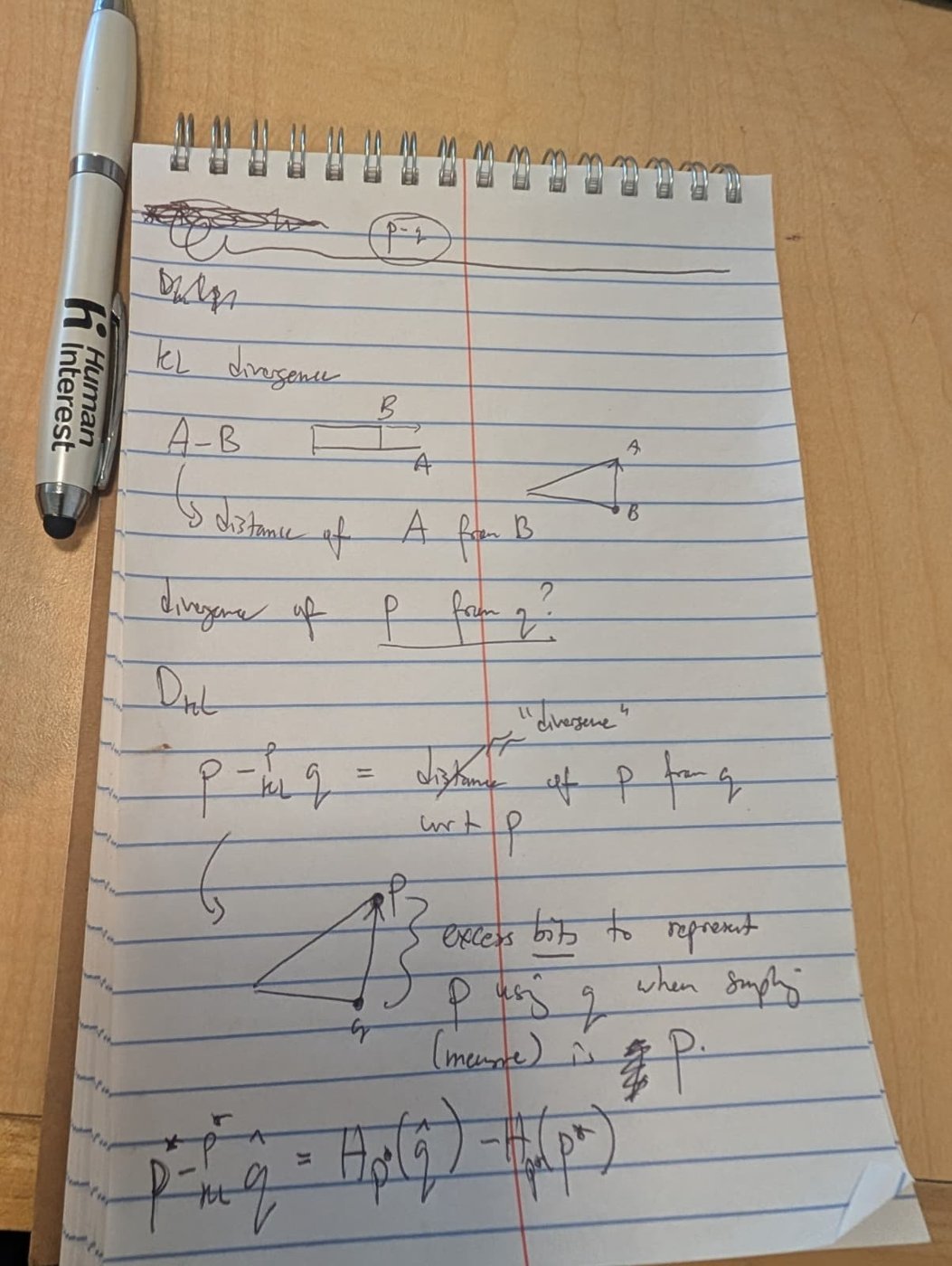
\[D_{\mathrm{KL}}(p \Vert q) \;=\; D^{\mathrm{KL}}_{p}(p \Vert q) \;=:\; p \mathbin{-^{\mathrm{KL}}_{p}} q\] \[p \mathbin{-^{\mathrm{KL}}_{p}} q \;=\; \Delta^{\mathrm{KL}}_{p}(p, q) \;=\; \Delta^{\mathrm{KL}}_{p}(q \to p) \;=\; \Delta^{\mathrm{KL}}_{p}(p \leftarrow q).\]Read it out loud: the KL divergence of \(p\) from \(q\), measured on samples from \(p\). The \(\Delta\) is for displacement, and “divergence” here just means an unsymmetric distance, difference or displacement. Baseline \(q\), destination \(p\), just like \(B - A\) has baseline \(A\). Usually \(p\) is the target (the data) and \(q\) is the model approximating it. The superscript says which kind of subtraction; the subscript says whose samples we average over, the measure we use as the ruler. Both arrows say the same thing read in opposite directions: start at \(q\), arrive at \(p\).
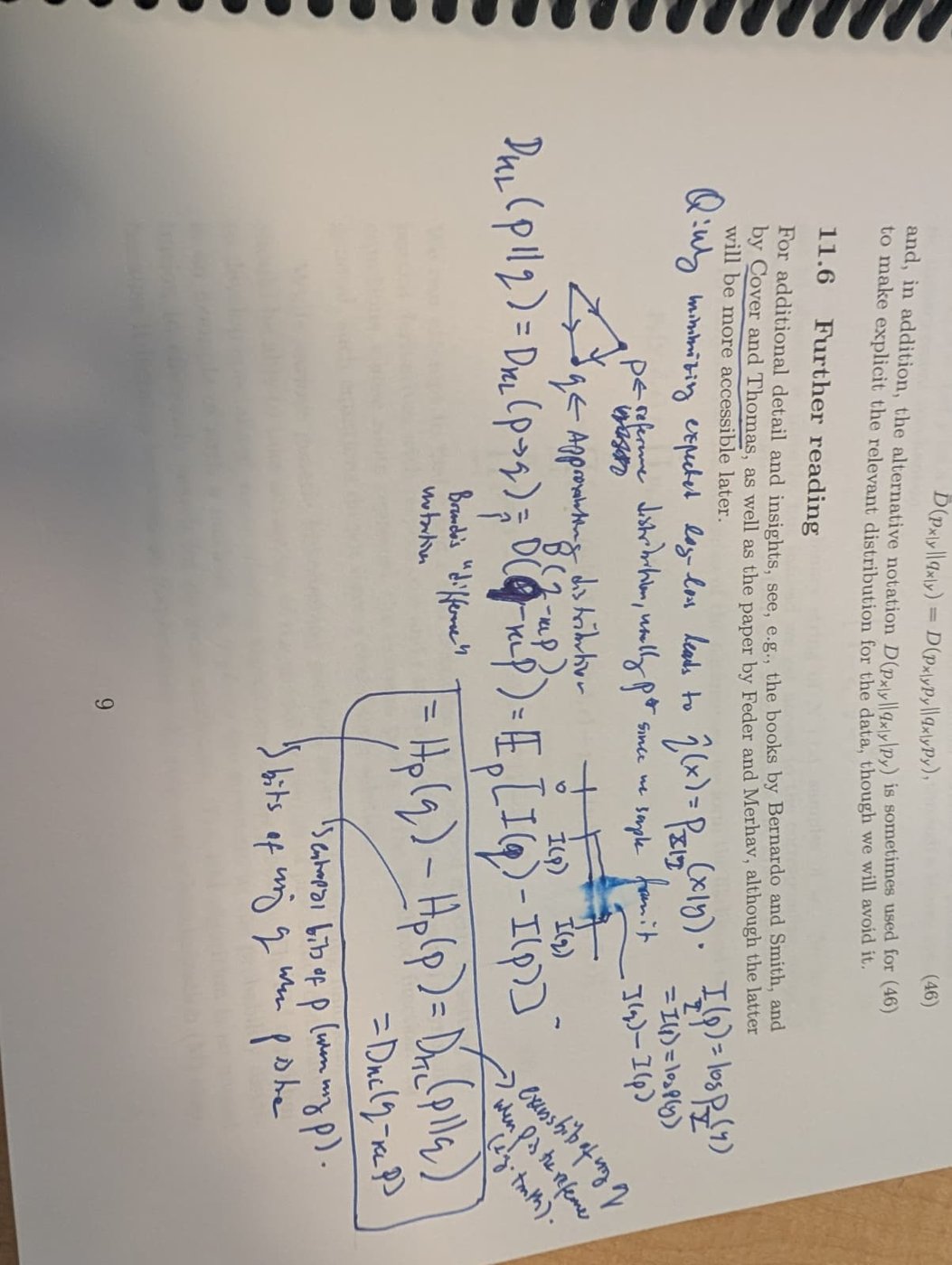
I’ll own a confusion here, because it’s exactly the one this notation prevents. On my first pass, in blue ink in the margin of a book chapter, I drew the arrow as \(p \to q\), as if \(p\) were “going to” \(q\). With the \(B - A\) grammar it is the other way around: in \(p \mathbin{-^{\mathrm{KL}}_{p}} q\), \(q\) is the starting point and we are measuring how far \(p\) sits from it. That’s why I thought my blue notes were wrong.
Put the two pictures side by side and the analogy is
\[p \mathbin{-^{\mathrm{KL}}_{p}} q \;=\; \mathbb{E}_{X \sim p}\big[\log p(X) - \log q(X)\big] \;\approx\; \text{“}A - B\text{”},\]the divergence of \(p\) from \(q\) next to the distance of \(A\) from \(B\). It’s a slight abuse of notation, which is why “\(A - B\)” is in quotes: \(p \mathbin{-^{\mathrm{KL}}_{p}} q\) is not a vector, it’s a scalar, like the Euclidean distance \(\Vert A - B \Vert_2\). Unlike that distance it is asymmetric, and the direction lives in the subscript.
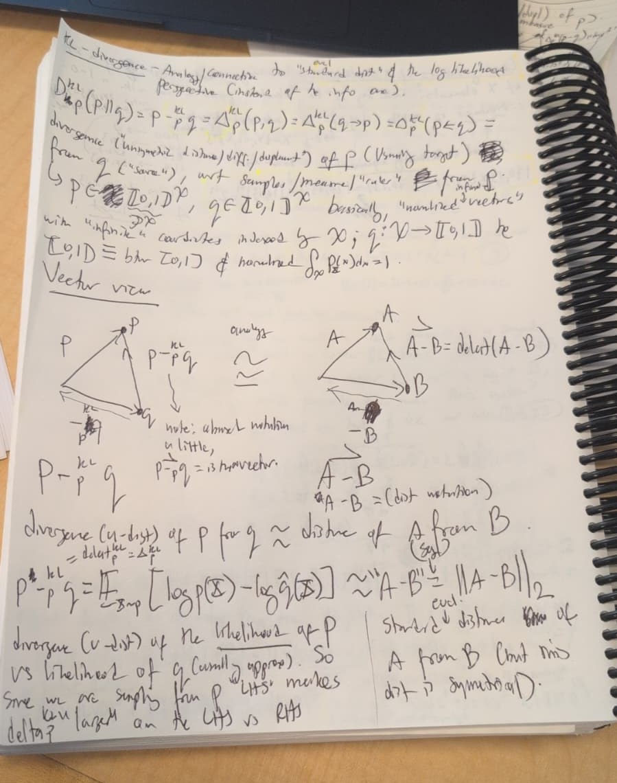
A note on the margin question on that page, since you might have the same one: does sampling from \(p\) make \(\log p(X)\) the bigger side? On average, yes: \(\mathbb{E}_p[\log p(X) - \log q(X)] \ge 0\) by Gibbs’ inequality (one line, in the next section). Not sample by sample: a particular \(x\) drawn from \(p\) can still be likelier under \(q\).
Unroll it: KL really is a subtraction
Write the definition out and the subtraction is sitting right there:
\[p \mathbin{-^{\mathrm{KL}}_{p}} q \;=\; \mathbb{E}_{X \sim p}\big[\, \log p(X) \;-\; \log q(X) \,\big].\]Define the pointwise log-likelihood displacement
\[\ell(x) \;:=\; \log p(x) - \log q(x).\]Then KL is just \(\mathbb{E}_p[\ell(X)]\). As a procedure:
- Sample \(x \sim p\).
- Score it under both models: \(\log p(x)\) and \(\log q(x)\).
- Subtract. That’s how much likelier \(p\) makes this \(x\) than \(q\) does, in log units (nats with \(\ln\), bits with \(\log_2\)).
- Average over many samples.
So \(D_{\mathrm{KL}}(p \Vert q)\) is the average log-likelihood advantage that \(p\) has over \(q\) on \(p\)’s own data. No minus signs to keep track of, no codes. A difference of two log-likelihoods, averaged.
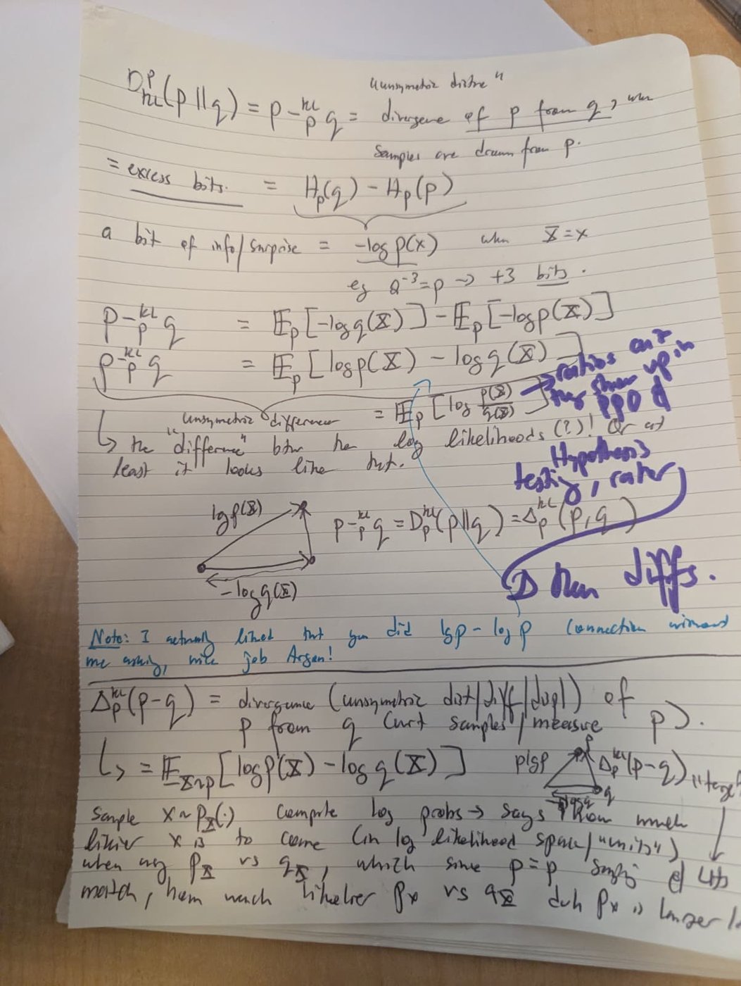
Two things are worth checking against the \(B - A\) picture.
Nonnegative, zero only at equality. For a particular \(x\), \(\ell(x)\) can be negative: \(q\) can like some of \(p\)’s samples more than \(p\) does. But on average, on \(p\)’s turf, \(p\) always wins or ties. That’s Gibbs’ inequality, one line of Jensen:
\[-\,\mathbb{E}_p[\ell(X)] \;=\; \mathbb{E}_p\!\left[\log \frac{q(X)}{p(X)}\right] \;\le\; \log \mathbb{E}_p\!\left[\frac{q(X)}{p(X)}\right] \;=\; \log 1 \;=\; 0,\]with equality only when \(p = q\) (almost everywhere).
Sometimes it literally is a distance. Take two Gaussians with the same variance, \(p = \mathcal{N}(\mu_p, \sigma^2)\) and \(q = \mathcal{N}(\mu_q, \sigma^2)\). Then
\[p \mathbin{-^{\mathrm{KL}}_{p}} q \;=\; \frac{(\mu_p - \mu_q)^2}{2\sigma^2},\]which is half the squared Euclidean distance between the means, in units of \(\sigma\). The displacement picture isn’t just a mnemonic; in the simplest case it is exactly the old distance.
Where the asymmetry lives
Here is the payoff. Swap \(p\) and \(q\) in the pointwise displacement and it flips sign, exactly like a vector:
\[\log q(x) - \log p(x) \;=\; -\,\ell(x).\]So the reverse KL is
\[q \mathbin{-^{\mathrm{KL}}_{q}} p \;=\; \mathbb{E}_{X \sim q}\big[-\ell(X)\big].\]Same pointwise displacement, opposite sign, different averaging distribution. In Euclidean space the norm forgets the sign and you get symmetry for free. In KL the “norm” is an average, and the average is taken under one of the two endpoints. Change the endpoint you sample from and you change the number. The asymmetry is entirely about whose turf you sample on, which is exactly what the subscript in \(\mathbin{-^{\mathrm{KL}}_{p}}\) records.
A concrete case. Let \(p = \mathcal{N}(0, 1)\) (narrow) and \(q = \mathcal{N}(0, 2^2)\) (wide). Then
\[p \mathbin{-^{\mathrm{KL}}_{p}} q \;\approx\; 0.32 \text{ nats}, \qquad q \mathbin{-^{\mathrm{KL}}_{q}} p \;\approx\; 0.81 \text{ nats}.\]On \(p\)’s data, the wide \(q\) is a bit diffuse but never shocked: cheap. On \(q\)’s data, the narrow \(p\) keeps seeing samples out in the tails that it thought were nearly impossible: expensive. This is the same fact behind “forward KL is mode-covering, reverse KL is mode-seeking,” and why maximum likelihood (forward) and variational inference (reverse) behave so differently. Fit a single Gaussian \(q\) to a two-mode \(p\) both ways and the subscript decides everything:
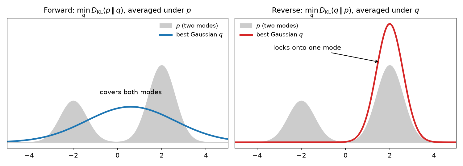
Averaged under \(p\) (left), any region where \(p\) has mass and \(q\) doesn’t costs a huge \(\ell(x)\), so \(q\) stretches to cover everything. Averaged under \(q\) (right), \(q\) only gets scored where it puts its own samples, so it’s free to ignore a whole mode. Koller and Friedman’s section on M- and I-projections (Section 8.5) is the cleanest treatment of this I know.
If you want a symmetric quantity, add the two directions (Jeffreys’ divergence):
\[p \mathbin{-^{\mathrm{KL}}_{p}} q \;+\; q \mathbin{-^{\mathrm{KL}}_{q}} p \;=\; \int \big(p(x) - q(x)\big)\big(\log p(x) - \log q(x)\big)\, dx .\]I like this identity a lot: a difference in probability space times a difference in log space. Both subtractions are visible at once.
How KL is and isn’t like a distance
Putting it side by side with the thing we started from:
| Half squared Euclidean, \(\tfrac12 \Vert B - A \Vert^2\) | KL, \(p \mathbin{-^{\mathrm{KL}}_{p}} q\) | |
|---|---|---|
| Pointwise displacement | \(B - A\) | \(\log p(x) - \log q(x)\) |
| Swapping the endpoints | flips the displacement’s sign | flips the displacement’s sign |
| Nonnegative, zero only at equality | yes | yes (Gibbs) |
| Symmetric | yes | no: the average is under one endpoint |
| Triangle inequality | no (the unsquared distance has it) | no |
| Bregman divergence generated by | \(\tfrac12 \Vert x \Vert^2\) | negative entropy \(\sum_x p(x) \log p(x)\) |
| Locally, near equality | itself | \(\tfrac12\, \delta^\top F(\theta)\, \delta\), with \(F\) the Fisher information |
The honest summary: KL is not a distance, but it behaves like half a squared distance. It belongs to the same family (Bregman divergences) as squared Euclidean distance. Nearby distributions see a quadratic form: \(D_{\mathrm{KL}}(p_\theta \Vert p_{\theta + \delta}) \approx \tfrac12 \delta^\top F(\theta) \delta\), so locally it is a squared length in the Fisher metric. It even has a Pythagorean identity for projections onto nice families of distributions (Csiszár, 1975). What it gives up is symmetry, and now we know exactly why.
Why I’d teach the log-likelihood view first
Three reasons.
The signs make sense. The bits view counts cost, so it is built from \(-\log\) terms, and KL becomes cost minus cost with sign flips you have to babysit. The log-likelihood view counts plausibility: bigger is better, and KL is the plausibility gap. Same number, no babysitting.
Maximum likelihood falls out in one line. If \(p\) is the data distribution and \(q_\theta\) is your model,
\[p \mathbin{-^{\mathrm{KL}}_{p}} q_\theta \;=\; \underbrace{\mathbb{E}_p[\log p(X)]}_{\text{does not depend on } \theta} \;-\; \mathbb{E}_p[\log q_\theta(X)].\]Minimizing over \(\theta\) is maximizing the expected log-likelihood, and with samples you replace \(\mathbb{E}_p\) by an average over your dataset. Maximum likelihood is minimizing the forward KL from the data to the model. In the displacement grammar: you are moving the baseline \(q_\theta\) toward the data, scored on the data’s own samples.
It connects to the rest of statistics. \(\ell(x)\) is the log-likelihood ratio, the central object of hypothesis testing, Bayesian evidence, importance sampling, and policy-gradient RL. Once KL is “average \(\ell\),” a lot of ML stops looking like a collection of unrelated tricks. That’s Appendix A.
Where this view came from, and why I’d never seen it
I didn’t get this from a course or a textbook. I got it while working through these notes with an AI model (Gemini): I was asking about the excess-bits formula, and it rewrote KL as \(\mathbb{E}_p[\log p - \log q]\) without my asking. It clicked immediately, and my honest reaction was: fourteen years, and nobody ever showed me it like this?
So I went looking for whether it’s new. It isn’t, as math. Kullback and Leibler (1951) introduced the quantity as “the mean information for discrimination” between two hypotheses “per observation from” one of them, which is precisely the expected log-likelihood ratio, and Kullback (1959) preferred the name discrimination information. Akaike (1973) built AIC on the same reading, and Wikipedia’s article has a whole “statistics” interpretation along these lines. There are good blog posts that lead with it too, like Alex Etz’s 2018 notes: KL is “the expected log likelihood ratio in favor of the true distribution.” Statisticians have had this view for 75 years.
Then I went through my own shelf: the books I was assigned or recommended at UIUC, MIT and Stanford, plus the notes from the MIT courses I took (photos of every book, and links to the notes, are in Appendix C). The subtraction is in almost all of them. What changes is what they tell you it means:
| Book or course notes | Writes KL as an expected log-difference or log-ratio? | Sampled log-likelihood form? | Headline intuition | Where |
|---|---|---|---|---|
| Hogg, McKean & Craig, Introduction to Mathematical Statistics (7th ed.) (photo) | Yes, unnamed: \(\mathbb{E}_{\theta_0}\big[\log \tfrac{f(X;\theta)}{f(X;\theta_0)}\big]\) | Yes: the average log-likelihood ratio over the sample | None: KL is never named there | Theorem 6.1.1 and its proof |
| MacKay, Information Theory, Inference, and Learning Algorithms (photo) | Yes, ratio form \(\sum_x P(x) \log \tfrac{P(x)}{Q(x)}\) | Partly: expected “weight of evidence” when codebreaking, not linked back to KL | Wasted bits | Sec. 2.6 (eq. 2.45); ch. 5 (p. 102); Secs. 18.3–18.4 |
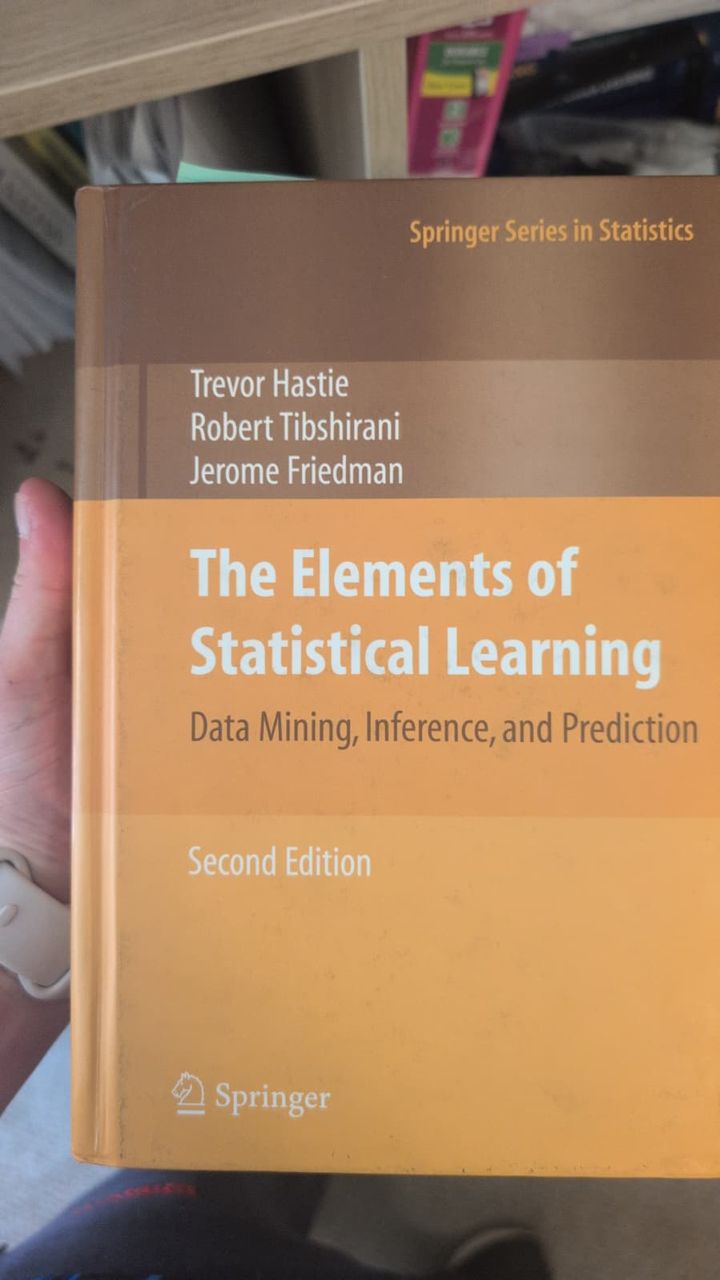
| Hastie, Tibshirani & Friedman, The Elements of Statistical Learning (2nd ed.) (photo) | Only as ICA’s mutual information | No | Dependence between components | Sec. 14.7.2 |
| Koller & Friedman, Probabilistic Graphical Models (photo) | Yes, and a proof writes \(\mathbb{E}_P[\log P - \log P']\) | Yes: to the expected log-likelihood, then the log-likelihood of the data | Extra coding cost, “compression loss (in bits)” | Def. A.5 (App. A.1.3); Prop. 16.1 (Sec. 16.2.1); Sec. 17.2.5 |
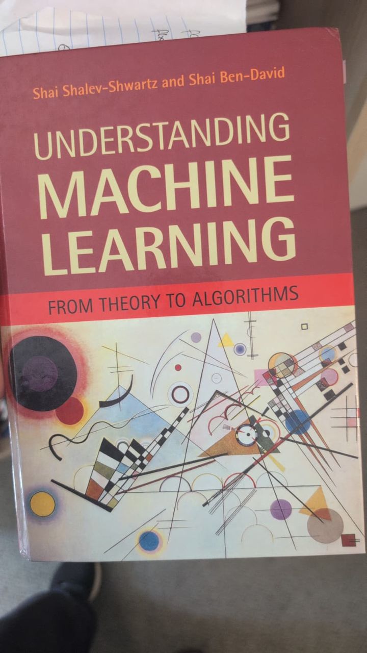
| Shalev-Shwartz & Ben-David, Understanding Machine Learning (photo) | Yes, ratio form, inside the true risk of the log-loss | Yes: maximum likelihood as ERM with the log-loss | Log-loss risk = relative entropy + entropy | Sec. 24.1 (eq. 24.5), 24.1.2 |
| Goodfellow, Bengio & Courville, Deep Learning (photo) | Yes, exactly \(\mathbb{E}_{x \sim P}[\log P(x) - \log Q(x)]\) | Yes: maximum likelihood as KL to the empirical distribution | Extra bits (nats) | Sec. 3.13 (eq. 3.50); Sec. 5.5 (eq. 5.60) |
| Bishop & Bishop, Deep Learning: Foundations and Concepts (photo) | As cross-entropy minus entropy, then \(-\int p \ln \tfrac{q}{p}\, dx\) | Not on that page; in exercise 2.34 | Additional information (nats) from coding with the wrong distribution | Sec. 2.5.5 (eq. 2.100) |
| Bishop, Pattern Recognition and Machine Learning (photo) | As cross-entropy minus entropy, then \(-\int p \ln \tfrac{q}{p}\, dx\) | Yes: \(\tfrac1N \sum_n \lbrace -\ln q(x_n \mid \theta) + \ln p(x_n) \rbrace\) | Additional information to transmit | Sec. 1.6.1 (eqs. 1.113, 1.119) |
| MIT 6.438 Algorithms for Inference, lecture notes, Fall 2014 (notes) | Ratio form \(\sum_x p(x) \log \tfrac{p(x)}{q(x)}\), as a bare definition | Yes: maximum likelihood as minimizing \(D(\hat p_{\mathcal D} \Vert p(\cdot\,;\theta))\), set against variational inference’s \(D(q \Vert p)\) | “How far apart two distributions are”, but not symmetric | Lec. 15–16 (p. 5); Lec. 20, Sec. 20.1.3 (p. 5) |
| MIT 6.867 Machine Learning, Jaakkola’s lecture notes (public version: Fall 2006) (notes) | No: never named in the 23 lectures | Only implicitly: EM’s lower bound on the log-likelihood, whose gap is a KL the notes never name | None | Lec. 16 (eq. 9, p. 4) |
Shalev-Shwartz and Ben-David come closest: KL first shows up as the excess log-loss risk, which is this view in cost form. Here is the coding version, from one of the newest books on my shelf, in the form I always had to stare at:
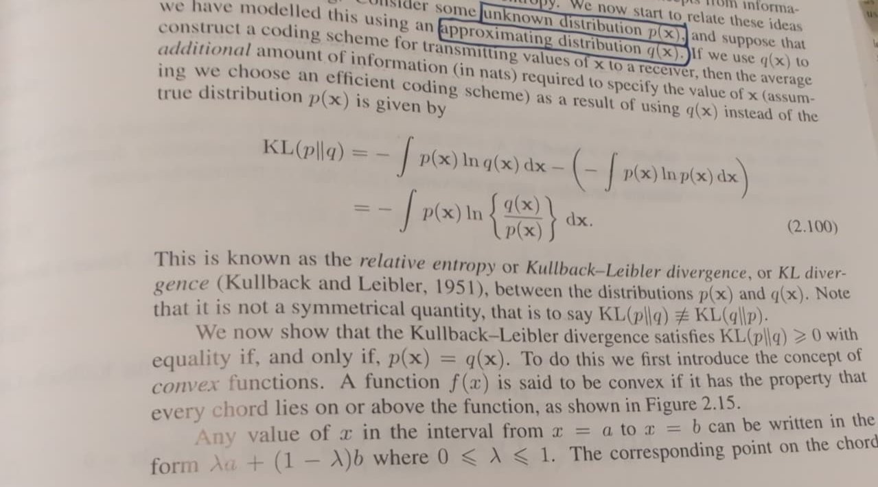
It’s completely correct. It just puts three minus signs and a coding story between me and the idea, and for years I re-derived which way the ratio goes every single time.
So the subtraction is written down in the standard books, sometimes even in its sampled form. What I could not find is any of them leading with it as the intuition: the headline is always bits. And I couldn’t find anyone folding it into one displacement grammar where the averaging distribution is part of the notation and explains the asymmetry. That part is my framing, and it’s the part I care about.
Why did it take me so long? My guess, and this is not a complaint about anyone: in a class, a talk, or a paper there’s a syllabus or a page limit, and “wait, why is it a ratio? why that sign?” feels like a question you’re supposed to already know the answer to. So it doesn’t get asked, and nobody stops to rebuild the foundations (I’ve written about that pressure before). I’m at a point where I’m happy to ask the basic question out loud and take the time to rebuild things. And AI changes the economics of that: a tireless sparring partner that never makes you feel slow. A curious person who works hard with AI can now understand the foundations more deeply than any course gave them. That’s the bet behind this series.
Appendix A: why ratios, and not differences?
Appendix: ~28 min read
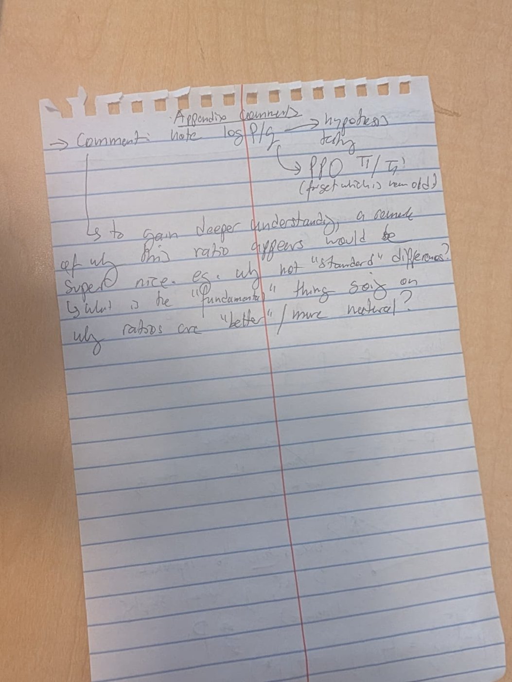
My note to myself was: what is the fundamental thing going on? Why are ratios more natural than standard differences? A few reasons, all of which are really the same reason, that \(\log p - \log q\) is the right subtraction for probabilities. A.1 is the short version; A.2 unpacks each point with the math and a small worked example.
A.1 The short version
- Evidence multiplies, so log-evidence adds up as subtractions. For \(n\) independent samples the likelihood ratio of the whole dataset is a product, \(\frac{p(x_1, \dots, x_n)}{q(x_1, \dots, x_n)} = \prod_i \frac{p(x_i)}{q(x_i)}\), and its log is a sum of subtractions, \(\sum_i \big[\log p(x_i) - \log q(x_i)\big] = \sum_i \ell(x_i)\): each sample adds one log subtraction. KL is that subtraction averaged per sample, \(D_{\mathrm{KL}}(p \Vert q) = \mathbb{E}_p[\log p(X) - \log q(X)]\). Raw differences \(p(x) - q(x)\) don’t compose across independent observations at all.
- Same answer in any units. Relabel \(x\) (meters to centimeters, \(x\) to \(\log x\), any smooth invertible \(y = g(x)\)) and both densities get multiplied by the same factor: \(p_Y(y) = p_X(x) \, \lvert dx/dy \rvert\) and \(q_Y(y) = q_X(x) \, \lvert dx/dy \rvert\). In the ratio a shared multiplicative factor cancels, \(p_Y(y)/q_Y(y) = p_X(x)/q_X(x)\), so KL doesn’t change. In the difference it stays: \(p_Y(y) - q_Y(y) = \big(p_X(x) - q_X(x)\big) \lvert dx/dy \rvert\).
- Bayes is additive in log-ratios. Posterior odds = prior odds × likelihood ratio, \(\frac{P(p \mid x)}{P(q \mid x)} = \frac{P(p)}{P(q)} \cdot \frac{p(x)}{q(x)}\), so one observation moves your log-odds toward \(p\) by exactly \(\ell(x) = \log p(x) - \log q(x)\) (Good and Turing called it weight of evidence).
- Hypothesis testing. By the Neyman–Pearson lemma, thresholding the likelihood ratio, “say \(p\) when \(\sum_i \ell(x_i) > t\)”, is the most powerful test between \(p\) and \(q\). And by Stein’s lemma, if you only allow a small fixed chance of rejecting \(p\) when it’s true, the best achievable chance of mistaking \(n\) samples from \(q\) for \(p\) decays like \(e^{-n D_{\mathrm{KL}}(p \Vert q)}\). KL is the exponent of distinguishability. (Kullback and Leibler’s paper is titled On Information and Sufficiency for a reason: the likelihood ratio is a sufficient statistic for telling \(p\) from \(q\).)
- Changing measure needs a ratio. Importance sampling: \(\mathbb{E}_p[f(X)] = \mathbb{E}_q\big[\tfrac{p(X)}{q(X)} f(X)\big]\). This is where PPO’s ratio comes from. It’s \(r_t(\theta) = \pi_\theta(a_t \mid s_t) / \pi_{\theta_{\text{old}}}(a_t \mid s_t)\), new over old (I always forget which way), and it reweights samples collected by the old policy so they score the new one. Its log is our subtraction for the two policies, \(\log r_t = \log \pi_\theta(a_t \mid s_t) - \log \pi_{\theta_{\text{old}}}(a_t \mid s_t)\), which is how code computes it: \(r_t = \exp(\log \pi_\theta - \log \pi_{\text{old}})\). The ratio is not itself a KL: averaged under the new policy, \(\log r\) gives \(D_{\mathrm{KL}}(\pi_\theta \Vert \pi_{\text{old}})\), and on the old policy’s samples, \(\mathbb{E}_{\text{old}}[-\log r]\) gives \(D_{\mathrm{KL}}(\pi_{\text{old}} \Vert \pi_\theta)\), the direction TRPO constrains. PPO’s clipping of \(r\) is a cheap trust region on that same pointwise quantity.
Differences of probabilities do give you real distances, for example total variation \(\tfrac12 \sum_x \lvert p(x) - q(x) \rvert\), and Pinsker’s inequality bounds it by KL: \(\mathrm{TV}(p, q) \le \sqrt{D_{\mathrm{KL}}(p \Vert q)/2}\). They just don’t have the properties above, which is why ratios keep showing up everywhere in ML.
A.2 The details
One running example for all five points, so the numbers can be checked by hand. Let \(p\) be a bent coin that lands heads 90% of the time and \(q\) a fair coin. In nats (natural log):
\[\ell(H) = \log \frac{0.9}{0.5} \approx 0.588, \qquad \ell(T) = \log \frac{0.1}{0.5} \approx -1.609,\] \[D_{\mathrm{KL}}(p \Vert q) = 0.9 \cdot 0.588 + 0.1 \cdot (-1.609) \approx 0.368, \qquad D_{\mathrm{KL}}(q \Vert p) = 0.5 \cdot (-0.588) + 0.5 \cdot 1.609 \approx 0.511.\]A head is mild evidence for the bent coin; a tail is strong evidence against it. Keep those four numbers in mind.
1. Evidence multiplies
The math. Take \(x_1, \dots, x_n\) independent. The probability of the whole dataset is a product under either model, so the ratio is a product of per-sample ratios:
\[\frac{p(x_1, \dots, x_n)}{q(x_1, \dots, x_n)} \;=\; \frac{\prod_i p(x_i)}{\prod_i q(x_i)} \;=\; \prod_{i=1}^n \frac{p(x_i)}{q(x_i)}.\]Where the log subtraction comes in. Two log rules do all the work: the log of a product is a sum, \(\log(ab) = \log a + \log b\), and the log of a ratio is a subtraction, \(\log(a/b) = \log a - \log b\). Apply the first to the product over samples and the second to each factor:
\[\log \prod_{i=1}^n \frac{p(x_i)}{q(x_i)} \;=\; \sum_{i=1}^n \log \frac{p(x_i)}{q(x_i)} \;=\; \sum_{i=1}^n \big[\log p(x_i) - \log q(x_i)\big] \;=\; \sum_{i=1}^n \ell(x_i).\]So “evidence multiplies” and “KL is a subtraction” are the same fact seen on two scales. On the probability scale, each new sample multiplies the evidence by \(p(x_i)/q(x_i)\). On the log scale, each new sample adds one subtraction, \(\log p(x_i) - \log q(x_i)\), to a running total. KL is the average size of that one subtraction: if the data really come from \(p\), the law of large numbers says \(\frac1n \sum_i \ell(x_i) \to \mathbb{E}_p[\log p(X) - \log q(X)] = D_{\mathrm{KL}}(p \Vert q)\). So the total evidence grows like \(n \cdot D_{\mathrm{KL}}(p \Vert q)\): KL is the rate at which evidence for \(p\) piles up, per sample, when \(p\) is the truth.
The example. Ten flips of the bent coin typically give 9 heads and 1 tail. The evidence is \(9(0.588) - 1.609 \approx 3.68 = 10 \times 0.368\) nats, so the data are \(e^{3.68} \approx 40\) times likelier under \(p\) than under \(q\). A hundred flips (90 heads) give \(36.8\) nats, a ratio of about \(10^{16}\).
Why the difference fails. Look at the same data through \(p(\text{data}) - q(\text{data})\). At 10 flips it’s \(0.0387 - 0.0010 \approx 0.038\). At 100 flips it’s \(7.6 \times 10^{-15} - 7.9 \times 10^{-31} \approx 7.6 \times 10^{-15}\). The evidence went from “40 to 1” to “\(10^{16}\) to 1” and the difference went down by thirteen orders of magnitude, because every specific long sequence is improbable under both models. The difference measures how small the probabilities are, not how much the data favor one model. The ratio throws away the part both models share and keeps exactly the part that discriminates.
2. Same answer in any units
What “coordinates” means here. The same random quantity can be written down in many ways: a height in meters or in centimeters, a positive number as \(x\) or as \(\log x\), a probability as itself or as its logit. These are relabelings. Nothing about the world changed, only the ruler you read it with. A comparison between two distributions should give the same answer whichever ruler you picked, and the log-ratio does. The pointwise difference doesn’t.
The Jacobian factor, written out. For a continuous variable, \(p(x)\) isn’t a probability, it’s a probability per unit of \(x\). Relabel with any smooth invertible \(y = g(x)\), so \(x = g^{-1}(y)\). The probability of a tiny interval can’t depend on which ruler measures it, so \(p_Y(y) \, \lvert dy \rvert = p_X(x) \, \lvert dx \rvert\), which gives
\[p_Y(y) \;=\; p_X\big(g^{-1}(y)\big) \left\lvert \frac{dx}{dy} \right\rvert \;=\; \frac{p_X(x)}{\lvert g'(x) \rvert}.\]That factor \(\lvert dx/dy \rvert = 1/\lvert g'(x) \rvert\) is the Jacobian: how much the new ruler stretches or squeezes space near \(x\). In \(d\) dimensions it’s \(\left\lvert \det \frac{\partial g^{-1}(y)}{\partial y} \right\rvert\). The key point is that it depends only on the relabeling \(g\) and the point, not on which distribution you’re transforming, so \(q\) gets exactly the same factor: \(q_Y(y) = q_X(x) \, \lvert dx/dy \rvert\).
Ratio: the factor cancels.
\[\frac{p_Y(y)}{q_Y(y)} \;=\; \frac{p_X(x) \, \lvert dx/dy \rvert}{q_X(x) \, \lvert dx/dy \rvert} \;=\; \frac{p_X(x)}{q_X(x)}, \qquad \text{so } \ell_Y(y) = \ell_X(x).\]Since \(y\) is just \(x\) relabeled, averaging that same number under \(p\) gives the same KL in either coordinate system.
Difference: the factor stays.
\[p_Y(y) - q_Y(y) \;=\; \big(p_X(x) - q_X(x)\big) \left\lvert \frac{dx}{dy} \right\rvert.\]The intuition. A ratio removes any multiplicative factor the two models share; a difference keeps it. The Jacobian is one such factor. The normalizer \(P(x)\) in Bayes’ rule (point 3) is another, and so is the \(\frac{1}{\sigma\sqrt{2\pi}}\) in front of two Gaussians with the same \(\sigma\). Whenever the two models are scaled by something that has nothing to do with which model is right, the ratio is the comparison that doesn’t see it.
The example. Heights: \(p = \mathcal{N}(1.70, 0.10^2)\) and \(q = \mathcal{N}(1.60, 0.10^2)\) in meters. At \(x = 1.70\) m, \(p_X = 3.989\) and \(q_X = 2.420\) per meter: ratio \(1.649\), difference \(1.570\). Now measure in centimeters, \(y = 100x\), so \(x = y/100\) and \(\lvert dx/dy \rvert = 1/100\). Both densities get multiplied by \(1/100\): \(p_Y = 0.03989\) and \(q_Y = 0.02420\) per centimeter. The ratio is still \(1.649\), while the difference fell 100-fold to \(0.0157\). The Gaussian formula from the main text agrees: in \(\frac{(\mu_p - \mu_q)^2}{2\sigma^2}\) the numerator and \(\sigma^2\) both grow by \(100^2\), so KL is \(\frac{0.1^2}{2 \times 0.01} = \frac{10^2}{2 \times 100} = 0.5\) nats either way. Units are a choice you made, not a fact about the two distributions, and the log-ratio is the pointwise comparison that can’t see that choice.
One honest caveat. Integrated differences are fine: \(\int \lvert p(x) - q(x) \rvert \, dx\) doesn’t depend on coordinates either, because the \(dx\) picks up the Jacobian back. The problem is only with the pointwise difference, and the pointwise comparison is what ML actually computes on samples. The pointwise log-ratio is meaningful on its own; the pointwise difference only becomes meaningful after you integrate it.
3. Bayes is additive in log-ratios
The math. Put a prior on the two hypotheses, \(P(p)\) and \(P(q)\). Bayes’ rule for each is \(P(p \mid x) = P(p) \, p(x) / P(x)\) and \(P(q \mid x) = P(q) \, q(x) / P(x)\). Divide one by the other and the shared normalizer \(P(x)\) cancels:
\[\frac{P(p \mid x)}{P(q \mid x)} \;=\; \frac{P(p)}{P(q)} \cdot \frac{p(x)}{q(x)}, \qquad \text{so} \qquad \log \frac{P(p \mid x)}{P(q \mid x)} \;=\; \log \frac{P(p)}{P(q)} \;+\; \ell(x).\]Posterior log-odds = prior log-odds + \(\ell(x)\). With \(n\) independent samples you just keep adding: \(+\,\ell(x_1) + \dots + \ell(x_n)\). So belief updating, on the log-odds scale, is addition of \(\ell\), and KL is the expected step toward \(p\) per sample when \(p\) is true. Notice also that the posterior depends on the data only through the ratio: multiply \(p(x)\) and \(q(x)\) by the same constant and nothing changes, while their difference would.
Where the name comes from. Turing used exactly this at Bletchley Park to score evidence about Enigma settings, in units he called bans (log base 10) and decibans (a tenth of that). I. J. Good, who worked with him, later wrote it up as weight of evidence.
The example. Start skeptical: prior odds 1 to 100 against the bent coin, about \(-4.6\) nats. Each head adds \(0.588\), each tail subtracts \(1.609\). If the coin really is bent you drift up by \(0.368\) per flip on average, so you reach even odds after about \(4.6 / 0.368 \approx 12.5\) flips. One tail costs you almost three heads’ worth of progress, which is the asymmetry of \(\ell\) showing up in practice.
4. Hypothesis testing
Neyman–Pearson. You want a rule that looks at the data and says “\(p\)” or “\(q\)”. Fix how often you’re willing to wrongly reject one of them. The lemma says the rule that minimizes the other error is: compute \(\frac{p(x)}{q(x)}\) and compare it to a threshold. With \(n\) samples that’s “is \(\sum_i \ell(x_i)\) above \(t\)?”. No other function of the data does better. That’s what sufficiency means here: once you know the likelihood ratio, nothing else in the data helps you tell \(p\) from \(q\).
Stein’s lemma. Now ask how fast the errors can shrink as \(n\) grows. Keep the chance of rejecting \(p\) when \(p\) is true below some small fixed \(\varepsilon\). Then the smallest achievable chance of the other mistake, saying “\(p\)” when the samples actually came from \(q\), behaves like
\[\beta_n \approx e^{-n \, D_{\mathrm{KL}}(p \Vert q)}.\]The intuition. To keep the first error small, the test says “\(p\)” whenever the evidence \(\sum_i \ell(x_i)\) is near its typical value under \(p\), about \(n D_{\mathrm{KL}}(p \Vert q)\). The second error happens when \(q\)’s samples happen to look like \(p\)’s, and by Sanov’s theorem the chance that \(n\) samples from \(q\) look like typical samples from \(p\) is about \(e^{-n D_{\mathrm{KL}}(p \Vert q)}\). So KL in this direction is “how hard is it for \(q\) to fake data from \(p\)”, and the average is under \(p\) because \(p\)’s typical data is what has to be faked.
The example. For a fair coin to fake the bent one it has to produce about 90% heads: with 20 flips that’s about \(e^{-20 \times 0.368} \approx 6 \times 10^{-4}\). For the bent coin to fake the fair one it has to produce about 50% tails, which it rarely does, so that’s harder: \(e^{-20 \times 0.511} \approx 4 \times 10^{-5}\). Two different numbers, because the two directions of KL answer two different questions. That’s the asymmetry from the main text, now as error rates. (These are rates; the exact probabilities carry slower-growing factors in front.)
5. Changing measure needs a ratio
The math. You want an average under \(p\), but your samples come from \(q\). Multiply and divide by \(q\):
\[\mathbb{E}_p[f(X)] \;=\; \sum_x p(x) f(x) \;=\; \sum_x q(x) \, \frac{p(x)}{q(x)} \, f(x) \;=\; \mathbb{E}_q\!\left[\frac{p(X)}{q(X)} f(X)\right],\]valid as long as \(q(x) > 0\) wherever \(p(x) f(x) \neq 0\). The weight \(p(x)/q(x)\) answers “how much more often would \(p\) have produced this \(x\) than \(q\) did?”, and that question has a ratio for an answer. Even an additive correction doesn’t escape it: \(\mathbb{E}_p[f] - \mathbb{E}_q[f] = \mathbb{E}_q\big[(\tfrac{p}{q} - 1) f\big]\), so estimating the difference from \(q\)’s samples still needs the ratio. KL itself can be computed this way: \(D_{\mathrm{KL}}(p \Vert q) = \mathbb{E}_q\big[\tfrac{p}{q} \log \tfrac{p}{q}\big]\).
The example. Flip the fair coin and weight each head by \(0.9/0.5 = 1.8\) and each tail by \(0.1/0.5 = 0.2\). The weighted fraction of heads is \(0.5 \times 1.8 = 0.9\): you’ve measured the bent coin using only fair-coin flips.
PPO, slowly: why the ratio is there
PPO’s objective has \(r_t(\theta) = \pi_\theta(a_t \mid s_t) / \pi_{\theta_{\text{old}}}(a_t \mid s_t)\) in it, and it’s easy to accept it without seeing why. The one-line answer: the data was collected by the old policy, but you’re scoring the new one, and the ratio is the importance weight that converts one into the other. Below is the whole chain, one step at a time. The equations follow Schulman et al.’s PPO paper (2017) and TRPO paper (2015); “PPO eq. 6” means equation 6 in their paper.
Step 1: what we’re maximizing. A policy \(\pi_\theta(a \mid s)\) picks actions, and \(\eta(\pi)\) is its expected discounted return. The advantage \(A_\pi(s, a) = Q_\pi(s, a) - V_\pi(s)\) says how much better action \(a\) is than what \(\pi\) does on average in state \(s\), so \(\mathbb{E}_{a \sim \pi}[A_\pi(s, a)] = 0\) in every state. To push \(\pi_\theta\) toward good actions, take the gradient of their average advantage. Fix a state and hold the advantages fixed:
\[\nabla_\theta \, \mathbb{E}_{a \sim \pi_\theta}[A(a)] \;=\; \sum_a \nabla_\theta \pi_\theta(a) \, A(a) \;=\; \sum_a \pi_\theta(a) \, \nabla_\theta \log \pi_\theta(a) \, A(a) \;=\; \mathbb{E}_{a \sim \pi_\theta}\big[\nabla_\theta \log \pi_\theta(a) \, A(a)\big],\]using \(\nabla \pi = \pi \, \nabla \log \pi\). Averaged over the states the policy visits, this is the policy gradient estimator \(\hat g = \hat{\mathbb{E}}_t\big[\nabla_\theta \log \pi_\theta(a_t \mid s_t) \, \hat A_t\big]\) (PPO eq. 1), the gradient of \(L^{PG}(\theta) = \hat{\mathbb{E}}_t\big[\log \pi_\theta(a_t \mid s_t) \, \hat A_t\big]\) (PPO eq. 2). Here \(\hat{\mathbb{E}}_t\) is an average over a batch of collected timesteps and \(\hat A_t\) is an estimate of the advantage.
Step 2: why the samples come from the old policy. That estimator is only right when the actions were sampled from \(\pi_\theta\) itself. But collecting data is the expensive part (running the simulator, the robot, the language model), so PPO runs \(\pi_{\theta_{\text{old}}}\) for a while, computes the \(\hat A_t\), and then takes many gradient steps on that one batch: \(K\) epochs of minibatch SGD (PPO Algorithm 1). After the first step, \(\theta \neq \theta_{\text{old}}\), but every sample in the batch still came from \(\pi_{\text{old}}\). Reusing \(L^{PG}\) anyway is, in the paper’s words, “not well-justified, and empirically it often leads to destructively large policy updates” (PPO §2.1). You can see exactly what goes wrong. On old data the gradient of \(L^{PG}\) is \(\sum_a \pi_{\text{old}}(a) \, \nabla_\theta \log \pi_\theta(a) \, A(a)\), while the gradient you wanted is \(\sum_a \pi_\theta(a) \, \nabla_\theta \log \pi_\theta(a) \, A(a)\). The weights are off by a factor of \(\pi_\theta(a) / \pi_{\text{old}}(a)\). That factor is the ratio.
Step 3: importance sampling puts the ratio in. Point 5’s identity, with \(p = \pi_\theta\) and \(q = \pi_{\text{old}}\), in one state \(s\):
\[\mathbb{E}_{a \sim \pi_\theta}\big[A(s, a)\big] \;=\; \sum_a \pi_\theta(a \mid s) \, A(s, a) \;=\; \sum_a \pi_{\text{old}}(a \mid s) \, \frac{\pi_\theta(a \mid s)}{\pi_{\text{old}}(a \mid s)} \, A(s, a) \;=\; \mathbb{E}_{a \sim \pi_{\text{old}}}\big[r(\theta) \, A(s, a)\big].\]It holds for every \(\theta\), not just at the start, as long as \(\pi_{\text{old}}(a \mid s) > 0\) wherever \(\pi_\theta(a \mid s) > 0\) (true for the usual softmax and Gaussian policies). Averaged over the batch, that’s the surrogate objective
\[L^{CPI}(\theta) \;=\; \hat{\mathbb{E}}_t\!\left[\frac{\pi_\theta(a_t \mid s_t)}{\pi_{\theta_{\text{old}}}(a_t \mid s_t)} \, \hat A_t\right] \;=\; \hat{\mathbb{E}}_t\big[r_t(\theta) \, \hat A_t\big] \qquad \text{(PPO eq. 6)}.\]CPI stands for conservative policy iteration (Kakade and Langford, 2002), where this objective was proposed. TRPO eq. 14 writes the same thing with a general sampling distribution \(q(a \mid s)\) in the denominator and \(Q\)-values in place of advantages. So the ratio is the reason one batch can be reused: it lets old samples estimate how the new policy would do, at whatever \(\theta\) the optimizer has reached.
What the ratio fixes and what it doesn’t. The exact improvement from switching policies is (Kakade and Langford’s identity, TRPO eq. 1, rewritten as a sum over states in TRPO eq. 2)
\[\eta(\tilde\pi) \;=\; \eta(\pi) + \sum_s \rho_{\tilde\pi}(s) \sum_a \tilde\pi(a \mid s) \, A_\pi(s, a),\]where \(\rho_{\tilde\pi}\) is how often the new policy visits each state. TRPO’s surrogate (TRPO eq. 3) swaps that for the old policy’s visits:
\[L_\pi(\tilde\pi) \;=\; \eta(\pi) + \sum_s \rho_{\pi}(s) \sum_a \tilde\pi(a \mid s) \, A_\pi(s, a).\]The ratio corrects the actions exactly. The states stay uncorrected, because your batch only has states the old policy reached. Why not correct those too? The weight for a whole trajectory is a product of per-step ratios, \(\prod_t \pi_\theta(a_t \mid s_t) / \pi_{\text{old}}(a_t \mid s_t)\). Evidence multiplies again (point 1), and products of many ratios blow up: a ratio of just \(1.1\) per step over 100 steps is \(1.1^{100} \approx 13{,}800\). So TRPO and PPO correct only the action at each step and keep the new policy close enough to the old one that the states it visits barely change. That’s the main theoretical reason for the trust region; noisy advantage estimates (step 5) are the practical one.
Step 4: at the start, the ratio’s gradient is the policy gradient. The denominator \(\pi_{\text{old}}(a_t \mid s_t)\) is a number saved during data collection, so it’s a constant:
\[\nabla_\theta r_t(\theta) \;=\; \frac{\nabla_\theta \pi_\theta(a_t \mid s_t)}{\pi_{\text{old}}(a_t \mid s_t)} \;=\; \frac{\pi_\theta(a_t \mid s_t)}{\pi_{\text{old}}(a_t \mid s_t)} \, \nabla_\theta \log \pi_\theta(a_t \mid s_t) \;=\; r_t(\theta) \, \nabla_\theta \log \pi_\theta(a_t \mid s_t).\]At \(\theta = \theta_{\text{old}}\), \(r_t = 1\), so
\[\nabla_\theta L^{CPI}(\theta) \Big\vert_{\theta_{\text{old}}} \;=\; \hat{\mathbb{E}}_t\big[\nabla_\theta \log \pi_\theta(a_t \mid s_t) \big\vert_{\theta_{\text{old}}} \, \hat A_t\big] \;=\; \hat g.\]The first gradient PPO computes is exactly the vanilla policy gradient \(\hat g\). From the second step on, the two differ: each sample’s gradient gets multiplied by its current \(r_t\), which is precisely the correction step 2 said was missing. In code, the ratio is computed as our subtraction, exponentiated: ratio = exp(logp_new - logp_old), with logp_old stored from the rollout. So \(\log r_t = \log \pi_\theta(a_t \mid s_t) - \log \pi_{\text{old}}(a_t \mid s_t)\) is the \(\ell\) of this post, per sample, for the two policies.
Step 5: why clip, and what the min does. \(L^{CPI}\) is linear in \(r_t\). Nothing stops the optimizer from pushing a good action’s ratio to 5 or 50, and “without a constraint, maximization of \(L^{CPI}\) would lead to an excessively large policy update” (PPO §3), far outside the region where the uncorrected states and the noisy \(\hat A_t\) can be trusted. PPO’s fix (PPO eq. 7, with \(\epsilon = 0.2\) in the paper):
\[L^{CLIP}(\theta) \;=\; \hat{\mathbb{E}}_t\Big[\min\big(r_t(\theta) \, \hat A_t,\ \mathrm{clip}(r_t(\theta), 1 - \epsilon, 1 + \epsilon) \, \hat A_t\big)\Big].\]Take one term, write \(c = \mathrm{clip}(r, 1 - \epsilon, 1 + \epsilon)\), and work the two signs of \(A\) separately.
- \(A > 0\) (a good action). Pull out the positive \(A\): \(\min(rA, cA) = A \cdot \min(r, c)\). If \(r \le 1 + \epsilon\), then \(\min(r, c) = r\) (below \(1 - \epsilon\), \(c = 1 - \epsilon > r\); in the middle, \(c = r\)). If \(r > 1 + \epsilon\), then \(c = 1 + \epsilon < r\) and the min is \(1 + \epsilon\). So the term is \(A \cdot \min(r, 1 + \epsilon)\): it rises with \(r\) up to \(1 + \epsilon\) and then goes flat. No reward for making a good action more than 1.2 times as likely as before, but if an update made it less likely, the full penalty stays and the gradient pulls it back.
- \(A < 0\) (a bad action). Pulling out a negative number flips min to max: \(\min(rA, cA) = A \cdot \max(r, c)\). If \(r \ge 1 - \epsilon\), then \(\max(r, c) = r\) (above \(1 + \epsilon\), \(c = 1 + \epsilon < r\)). If \(r < 1 - \epsilon\), then \(c = 1 - \epsilon > r\) and the max is \(1 - \epsilon\). So the term is \(A \cdot \max(r, 1 - \epsilon)\): flat once the bad action is below 0.8 times its old probability, but if an update made it more likely, the full penalty stays.
- \(A = 0\). The term is 0 whatever \(r\) is.
That’s the paper’s Figure 1, and its own summary: “we only ignore the change in probability ratio when it would make the objective improve, and we include it when it makes the objective worse.” Since \(\min(r, 1 + \epsilon) \le r\) when \(A > 0\) and \(\max(r, 1 - \epsilon) \ge r\) when \(A < 0\), every clipped term is \(\le r_t \hat A_t\): \(L^{CLIP}\) is a pessimistic lower bound on \(L^{CPI}\), and the two agree to first order around \(r = 1\). One honest detail: in the flat region the gradient is zero, so a sample stops pushing. It doesn’t pull the policy back. The clip is a soft fence, which is why some implementations also watch the KL from step 6 and stop the epochs early when it gets too big.
Step 6: the trust-region family, and where KL comes in. TRPO (PPO eqs. 3–4, TRPO eq. 14) keeps the unclipped surrogate and adds a hard constraint:
\[\max_\theta \ \hat{\mathbb{E}}_t\big[r_t(\theta) \, \hat A_t\big] \quad \text{subject to} \quad \hat{\mathbb{E}}_t\Big[D_{\mathrm{KL}}\big(\pi_{\text{old}}(\cdot \mid s_t) \,\Vert\, \pi_\theta(\cdot \mid s_t)\big)\Big] \le \delta.\]The theory behind it (TRPO Theorem 1 and eq. 9) is a lower bound on the true return, \(\eta(\tilde\pi) \ge L_\pi(\tilde\pi) - C \max_s D_{\mathrm{KL}}\big(\pi(\cdot \mid s) \Vert \tilde\pi(\cdot \mid s)\big)\) with \(C = \frac{4 \varepsilon \gamma}{(1 - \gamma)^2}\) and \(\varepsilon = \max_{s, a} \lvert A_\pi(s, a) \rvert\) (a different \(\varepsilon\) from PPO’s clip). Maximize the right-hand side and the true return can’t go down. That bound suggests a penalty, and PPO’s other variant (PPO eq. 8) uses one: \(\hat{\mathbb{E}}_t\big[r_t \hat A_t - \beta \, D_{\mathrm{KL}}(\pi_{\text{old}}(\cdot \mid s_t) \Vert \pi_\theta(\cdot \mid s_t))\big]\), halving \(\beta\) when the measured KL is below \(d_{\text{targ}}/1.5\) and doubling it when it’s above \(1.5 \, d_{\text{targ}}\). Clipping needs neither a KL computation nor TRPO’s conjugate-gradient solve, just SGD or Adam on one loss. In the paper’s MuJoCo comparison (Table 1, normalized so random = 0 and best = 1), no clipping or penalty scored \(-0.39\), clipping with \(\epsilon = 0.2\) scored \(0.82\), and the best adaptive-KL setting scored \(0.74\).
The KL in all of these is \(D_{\mathrm{KL}}(\pi_{\text{old}} \Vert \pi_\theta) = \mathbb{E}_{a \sim \pi_{\text{old}}}\big[\log \pi_{\text{old}}(a \mid s) - \log \pi_\theta(a \mid s)\big] = \mathbb{E}_{\text{old}}[-\log r]\): our subtraction averaged on the old policy’s turf, which is the direction you can estimate by plainly averaging over the batch you have, with no reweighting. Because \(\mathbb{E}_{\text{old}}[r] = 1\), the same KL is also \(\mathbb{E}_{\text{old}}\big[(r - 1) - \log r\big]\), and that version is never negative sample by sample, so it’s the low-variance estimator many RL codebases log. (Averaged instead on the new policy’s samples, \(\log r\) gives \(D_{\mathrm{KL}}(\pi_\theta \Vert \pi_{\text{old}})\), the other direction.) TRPO bounds the old-policy average of \(-\ell\); PPO clips \(r = e^{\ell}\) itself, sample by sample. Same pointwise quantity, two ways to keep it on a leash.
Step 7: a small example you can check by hand. One state, two actions. Under the old policy the good action \(g\) has probability \(0.2\) and advantage \(+1\); the bad action \(b\) has probability \(0.8\) and advantage \(-0.25\). Check: \(0.2(1) + 0.8(-0.25) = 0\), as advantages under their own policy must average.
- One update moves \(g\) from \(0.2\) to \(0.3\) and \(b\) from \(0.8\) to \(0.7\). Ratios: \(r_g = 0.3/0.2 = 1.5\) and \(r_b = 0.7/0.8 = 0.875\).
- The truth. The new policy’s average advantage is \(0.3(1) + 0.7(-0.25) = 0.125\). In a one-step (bandit) problem that’s exactly how much the return went up.
- Old samples, no ratio. Averaging \(A\) over the old policy’s samples gives \(0.2(1) + 0.8(-0.25) = 0\), whatever \(\theta\) is. The batch can’t see that anything changed.
- Old samples, with the ratio. \(0.2(1.5)(1) + 0.8(0.875)(-0.25) = 0.3 - 0.175 = 0.125\). Exactly right.
- Clipped, \(\epsilon = 0.2\). For \(g\), \(A > 0\) and \(r = 1.5 > 1.2\), so its term is capped: \(0.2 \times 1.2 \times 1 = 0.24\). For \(b\), \(A < 0\) and \(r = 0.875\) is above \(0.8\), so it isn’t: \(0.8 \times 0.875 \times (-0.25) = -0.175\). \(L^{CLIP} = 0.065\), below \(L^{CPI} = 0.125\), as the lower bound says.
- Where the optimizer stops. Let \(p\) be the new probability of \(g\). The unclipped surrogate is \(1.25p - 0.25\), and it keeps climbing all the way to \(p = 1\), a deterministic policy, where \(D_{\mathrm{KL}}(\pi_{\text{old}} \Vert \pi_\theta) = \infty\). The clipped one goes flat at \(p = 0.36\): past there \(g\)’s term is capped at \(0.24\) and \(b\)’s ratio \((1-p)/0.8\) has dropped below \(0.8\). Gradient ascent stops there, at \(D_{\mathrm{KL}} \approx 0.061\) nats. For comparison, \(p = 0.3\) is at \(D_{\mathrm{KL}} \approx 0.026\), and a TRPO limit of \(\delta = 0.01\) would stop at \(p \approx 0.26\).
- Two lessons. First, at the stopping point \(r_g = 0.36/0.2 = 1.8\), well past \(1.2\): \(g\)’s own term stopped pushing at \(p = 0.24\), but \(b\)’s term kept lowering \(b\), and with two actions that raises \(g\). The clip limits each term’s incentive, not each ratio. Second, in this toy the advantages are exact and there’s only one state, so going all the way to \(p = 1\) would actually be right. In real RL, \(\hat A_t\) is a noisy estimate from one batch and the states shift as the policy moves, so a jump to a deterministic policy based on one batch is how training collapses. The ratio lets you reuse the batch; the clip keeps you near where the batch is still trustworthy.
Differences aren’t useless
Total variation is built from differences and it’s a perfectly good distance:
\[\mathrm{TV}(p, q) = \tfrac12 \sum_x \lvert p(x) - q(x) \rvert = \max_{A} \lvert P(A) - Q(A) \rvert,\]the biggest gap in probability the two models can disagree on for any single event. It’s symmetric, satisfies the triangle inequality and stays between 0 and 1. Pinsker’s inequality, \(\mathrm{TV}(p, q) \le \sqrt{D_{\mathrm{KL}}(p \Vert q)/2}\), says small KL forces small TV. For the coins: \(\mathrm{TV} = \lvert 0.9 - 0.5 \rvert = 0.4\) and \(\sqrt{0.368/2} \approx 0.43\), so the bound holds and is nearly tight. What TV can’t do is the four things above: it doesn’t add up over independent samples, it isn’t a per-sample Bayesian update, it isn’t the error exponent, and it can’t reweight samples.
The one reason underneath
Probabilities combine by multiplying: independent samples multiply, Bayes multiplies a prior by a likelihood, a change of variables multiplies by a Jacobian, reweighting multiplies by a weight. When the natural operation is multiplication, the natural comparison is division, and the log turns that division into a subtraction you can add up and average. So \(\log p - \log q\) isn’t a trick someone picked. It’s the subtraction that respects how probability actually composes, and KL is its average on \(p\)’s turf.
Appendix B: the classical bits view, side by side
The textbook route starts from surprisal. Seeing \(x\) with probability \(p(x)\) costs
\[-\log_2 p(x) \text{ bits}, \qquad \text{e.g. } p(x) = 2^{-3} \;\Rightarrow\; 3 \text{ bits}.\]Average it and you get entropy. Writing the sampling distribution as a subscript, as everywhere in this post:
\[H_p(q) \;:=\; \mathbb{E}_{X \sim p}[-\log q(X)] \quad \text{(cross-entropy)}, \qquad H_p(p) \;=\; \mathbb{E}_{X \sim p}[-\log p(X)] \quad \text{(entropy)}.\]\(H_p(q)\) is the expected code length when the data come from \(p\) but your code was built for \(q\); \(H_p(p)\) is the best you can do. Their difference is the classical reading of KL, the excess bits you waste by using the wrong code:
\[p \mathbin{-^{\mathrm{KL}}_{p}} q \;=\; H_p(q) - H_p(p) \;=\; \mathbb{E}_p[-\log q(X)] - \mathbb{E}_p[-\log p(X)] \;=\; \mathbb{E}_p[\log p(X) - \log q(X)].\]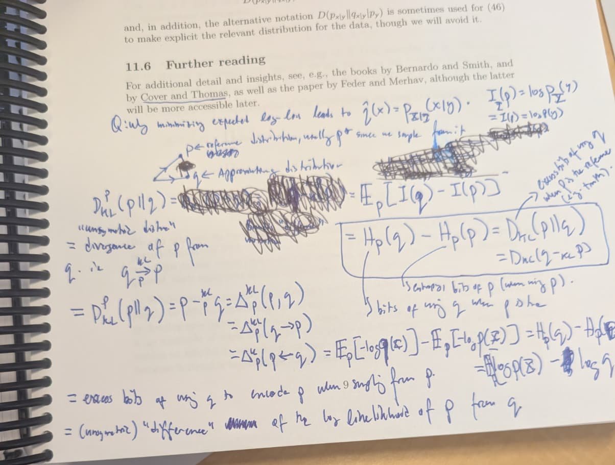
Same number, two ways of thinking:
- Bits view: a difference of costs. Bigger is worse, so everything carries a minus sign, and you subtract the optimal cost from the suboptimal one.
- Log-likelihood view: a difference of plausibilities. Bigger is better, no minus signs, and you subtract the baseline model’s log-likelihood from the true model’s, on the true model’s data.
The bits view is the right one when you actually care about compression. For learning, where everything we optimize is a log-likelihood anyway, I find the second one far easier to hold in my head. Use whichever builds your intuition, but know that they are the same subtraction.
Appendix C: the shelf
These are the eight books from the table, in the same order, photographed from my shelf. Each caption says in one line what the book does with KL; the sections and equation numbers are in the table.






The MIT course notes
I took three MIT courses where KL should come up: 6.437 (Inference and Information), 6.438 (Algorithms for Inference) and 6.867 (Machine Learning). Here is how their notes introduce it, using the public versions closest to when I took them:
- 6.438, Algorithms for Inference (lecture notes, Fall 2014, MIT OpenCourseWare). KL first appears in the Lecture 15–16 notes (p. 5), inside the variational characterization of \(\log Z\), as the bare ratio formula: “a way to measure how far apart two distributions are”, not a proper distance “because it is not symmetric.” The Lecture 20 notes (Sec. 20.1.3, p. 5) then show that maximum likelihood minimizes \(D(\hat p_{\mathcal D} \Vert p(\cdot\,;\theta))\), and point out that this optimizes the second argument, while variational inference optimized the first. That is the asymmetry from this post, said in two sentences and then left there.
- 6.867, Machine Learning (Tommi Jaakkola’s lecture notes; the public version is Fall 2006 on OCW). KL is never named in any of the 23 lectures. It is there implicitly in the Lecture 16 notes (eq. 9, p. 4): EM’s objective is the expected complete-data log-likelihood plus an entropy term, and it equals the log-likelihood exactly at the posterior. The gap between them is a KL divergence that the notes never call one.
- 6.437, Inference and Information (Golland and Wornell). I couldn’t find its lecture notes online; they don’t seem to be public. The course description lists “Log-loss inference criterion, entropy and model capacity. Kullback-Leibler distance and information geometry,” so KL sits right next to log-loss on the syllabus, but I can’t say how the notes framed it.
If you’d like to cite this post:
@misc{miranda2026klsubtraction,
  author = {Miranda, Brando},
  title  = {Reading KL Divergence as a Subtraction: Displacement, Asymmetry, and the Log-Likelihood View},
  year   = {2026},
  month  = {October},
  howpublished = {\url{https://cs.stanford.edu/people/brando9/2026/10/17/kl-divergence-as-a-subtraction.html}},
  note   = {Blog post}
}